Steps of the phylogenetic analysis

Compilation of sequence dataset

Alignment

Determination of substitution model

Tree building

Tree evaluation

Nucleotide Substitution Models

"All models are wrong but some are useful" (George Box, 1979)

As we have seen in Class 19, p-distance is not an accurate way to estimate a number of substitutions between two sequences.

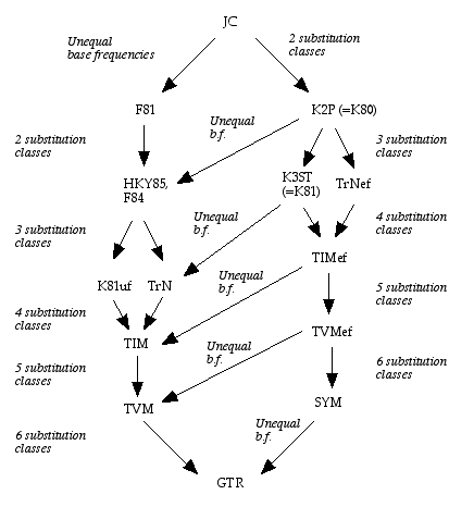
The simplest nucleotide substitution model is Jukes-Cantor model (a.k.a. JC69), which assumes that every nucleotide can be substituted with any other nucleotide with equal probability and all four bases occur with the same frequency (=0.25). This model has only one parameter (substitution rate α).

Fig. Nucleotide substitutions [Source].

If variable base composition allowed (usually estimated from the alignment), JC69 model is transformed into Felsenstein 1981 model (F81).

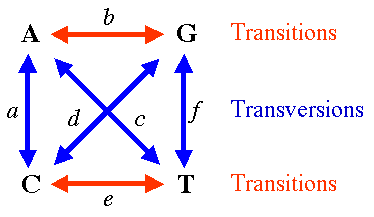
Table 7.2 in the supp. textbook gives a good summary of different substitution models for nucleotide sequences.

Alternatively, if transitions and transversions are distinguished, JC69 model becomes Kimura 2 parameter model (K2P or K80), two parameters being rates of transitions and transversions.

Hasegawa-Kishino-Yano 1985 model (HKY85) assumed both unequal base composition and different rates for transitions and transversions

General Time Reversible Model (GTR or REV) assumes unequal base frequencies and 6 different rates of nucleotide substitutions, i.e. each possible substitution has its own rate.

The models described above are related to each other (they are nested):

Fig. Nucleotide substitution models [Source].

Assumptions of the models:

All nucleotide sites change independently (counter-example: compensatory changes in rRNA)
The substitution rate is constant over time and in different lineages
The base composition within the dataset is the same (at equilibrium). [GC content of completed prokaryotic genomes]
All sites have the same constant probability to undergo substitution. [Among-Site-Rate-Variation, or ASRV, in later lectures.]

Choosing the right model: ModelTest

Protein Substitution Models

Protein Substitution Models are empirical (as opposed to parametric models for nucleotide substitutions described above). Examples: BLOSUM, PAM, JTT, WAG.

Fig. Protein substitution models [Source].

Reconstruction of Evolutionary History (Overview)

Distance analyses

calculate pairwise distances (different distance measures, correction for multiple hits, correction for codon bias)
make distance matrix (table of pairwise corrected distances)
calculate tree from distance matrix:
i) using optimality criterion (e.g.: smallest error between distance matrix and distances in tree)
ii) using algorithmic (or clustering) approaches (e.g., UPGMA or neighbor joining)

Parsimony analyses

find that tree that explains sequence data with minimum number of substitutions (tree includes hypothesis of sequence at each of the internal nodes). The underlying principle: Occam's Razor, i.e. the simplest solution is usually the correct one.

Maximum Likelihood (ML) analyses

given a model for sequence evolution, find the tree that has the highest probability (likelihood) of reproducing the observed data under this model. Likelihood describes how well the model predicts the data.

However, likelihood does not say anything about the probability of the model itself: Elliot Sober's Gremlins.

Bayesian analyses

use ML analyses to calculate posterior probabilities for trees, clades and evolutionary parameters.