CLASS 25. Bootstrapping. Long Branch Attraction. Concept of an Outgroup. Neighbor-Joining Trees.
Ch.11 (textbook);
Sections 8.4, 8.5 (supp. textbook);
Bootstrapping
|
Baron Karl Friedrich Hieronymus von Münchhausen |
Bootstrapping is one of the most popular ways to assess the reliability
of branches. The term bootstrapping
goes back to the Baron Münchhausen (who pulled himself out of a swamp
by his shoe laces). Briefly, positions of the aligned sequences are
randomly sampled from the multiple sequence alignment with replacements.
The sampled positions are assembled into new data sets, the
so-called bootstrapped samples. Each
position has an about 63% chance to make it into a particular bootstrapped
sample.If a grouping has a lot of support, it will
be supported by at least some positions in each of the bootstrapped
samples, and all the bootstrapped samples will yield this grouping.
Bootstrapping can be applied to all methods of phylogenetic reconstruction.
Bootstrapping has become very popular to assess the reliability of reconstructed phylogenies. Its advantage is that it can be applied to different methods of phylogenetic reconstruction, and that it assigns a probability-like number to every possible bipartition of the dataset (= branch in the resulting tree). Its disadvantage is that the support for individual groups decreases as you add more sequences to the dataset, and that it just measures how much support for a partition is in your data given a method of analysis. If the method of reconstruction falls victim to a bias or an artifact, this will be reproduced for every of the bootstrapped samples, and it will result in high bootstrap support values (see below). |

Creating a bootstrapped sample
Joe Felsenstein describes the bootstrap procedure in his manual to the seqboot program (part of the PHYLIP package, the manual is here, the citations here) as follows:
The bootstrap. Bootstrapping was invented by Bradley Efron in 1979, and its use in phylogeny estimation was introduced by me (Felsenstein, 1985b; see also Penny and Hendy, 1985). It involves creating a new data set by sampling N characters randomly with replacement, so that the resulting data set has the same size as the original, but some characters have been left out and others are duplicated. The random variation of the results from analyzing these bootstrapped data sets can be shown statistically to be typical of the variation that you would get from collecting new data sets. The method assumes that the characters evolve independently, an assumption that may not be realistic for many kinds of data.
The sample input and output of the seqboot program illustrates the generation of the bootstrapped samples:
TEST DATA SET
		    5    6
		Alpha     AACAAC
		Beta      AACCCC
		Gamma     ACCAAC
		Delta     CCACCA
		Epsilon   CCAAAC
CONTENTS OF OUTPUT FILE
(If Replicates are set to 10 and seed to 4333)
		    5     6
		Alpha        ACAAAC
		Delta        CACCCA
		Gamma        ACAAAC
		Beta         ACCCCC
		Epsilon      CAAAAC
		    5     6
		Alpha        AACAAC
		Beta         AACCCC
		Epsilon      CCAAAC
		Delta        CCACCA
		Gamma        CCCAAC
		    5     6
		Delta        CAACCC
		Beta         ACCCCC
		Gamma        ACCAAA
		Alpha        ACCAAA
		Epsilon      CAAAAA
		    5     6
		Alpha        AAAACA
		Beta         AAAACC
		Gamma        AAACCA
		Delta        CCCCAC
		Epsilon      CCCCAA
		    5     6
		Beta         ACCCCC
		Epsilon      CAAACC
		Delta        CCCCAA
		Gamma        AAAACC
		Alpha        AAAACC
		    5     6
		Gamma        CCAACC
		Alpha        ACAACC
		Epsilon      CAAACC
		Delta        CACCAA
		Beta         ACCCCC
		    5     6
		Alpha        AAACAA
		Delta        CCCACC
		Epsilon      CCCAAA
		Gamma        AACCAA
		Beta         AAACCC
		    5     6
		Alpha        AAAACC
		Delta        CCCCAA
		Beta         CCCCCC
		Epsilon      AAAACC
		Gamma        AAAACC
		    5     6
		Beta         AAAAAC
		Alpha        AAAAAC
		Gamma        AACCCC
		Delta        CCCCCA
		Epsilon      CCCCCC
		    5     6
		Delta        CCCCAA
		Epsilon      CCAACC
		Gamma        AAAACC
		Alpha        AAAACC
		Beta         AACCCC
Long Branch Attraction
In analyzing divergent sequences one frequently observed problem known as long-branch attraction (LBA). Even though the long branches might be closer related to short branches, many algorithms will group the long branches together. Although this problem has been extensively discussed in the literature, there is no easy solution to this problem.A similar case, although most algorithms are much less prone fall victim to this problem, is long branch attraction in cases where the substitution rate is the same in all lineages, but the long branches are due to the absence of side branches.
Parsimony is pretty sensitive, usually maximum likelihood approaches that incorporate among site rate variation (ASRV) into the model are doing pretty good. Distance analyses are somewhat in between (depending on the distance measure). Using simulated protein sequence evolution, i.e. the true tree is known for these sequences, we found (see poster ) that long-branch attraction in the presence of ASRV can become a problem even when sequences are more than 50% identical.
Outgroup
Trees from molecular data are usually calculated as unrooted trees (at least they should be - if they are not this is usually a mistake).
To root a tree you either can assume a molecular clock (substitutions occur at a constant rate, again this assumption is usually not warranted and needs to be tested), or you can use an outgroup (i.e. something that you know forms the deepest branch).
For example,
- to root a phylogeny of birds, you could use the homologous characters from a reptile as outgroup;
- to find the root in a tree depicting the relations between different human mitochondria, you could use the mitochondria from chimpanzees or from Neanderthals as an outgroup;
- to root a phylogeny of alpha hemoglobins you could use a beta hemoglobin sequence, or a myoglobin sequence as outgroup.
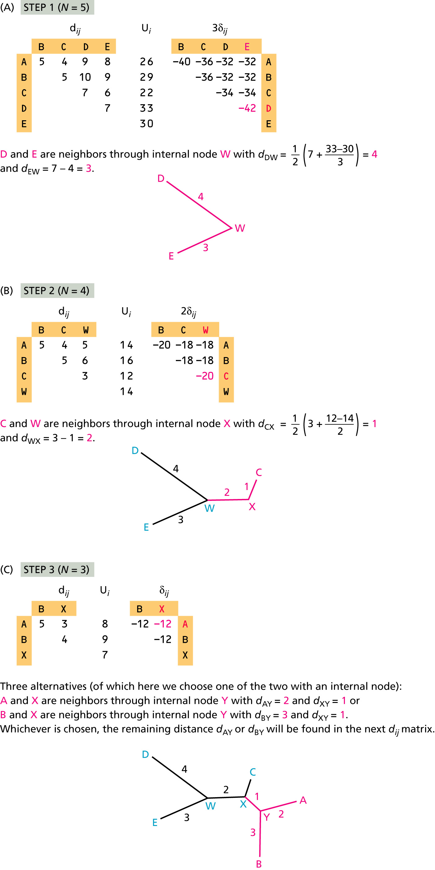
Neighbor-Joining Method
Neighbor Joining method (introduced by Naruya Saitou and Masatoshi Nei in 1987) is an approximate (and very fast) method to find a phylogenetic tree for which the total branch length of the tree is the shortest. The input for NJ method is a distance matrix.
Trees with CLUSTALX
Besides aligning sequences, ClustalX also includes programs to calculate distance trees. The trees generated by ClustalX certainly have their limitations, however, if one is aware of these limitations, the program is extremely useful for initial exploration.
Trees are calculated from a corrected or uncorrected distance matrix using the neighbor joining method.
Several parameters that you can choose in clustal influence tree building:
- The choice of substitution matrix, and other alignment parameters
- You can ignore all positions that in any of the sequences contains a gap
- You can correct for multiple substitutions (In a perfect world you want to use the actual number of substitutions that occurred in evolution, and not the number of sites that differ between two sequences).