Where to find genomes?
As of January 20, 2006 there are 2299 genome projects, of which 495 are completed and published
(Source: Genomes Online Database - GOLD).
Other places to look for genomic data:
- JGI (DOE Joint Genome Institute),
- NCBI Genomes (National Center for Biotechnology Information),
- Craig Venter Institute,
- TIGR Comprehensive Microbial Resource (CMR).
Vastness of Protein Space
The Size of Protein Sequence Space (back of the envelope calculation):
- Consider a protein of 600 amino acids.
- Assume that for every position there could be any of the twenty possible amino acid.
- Then the total number of possibilities is 20 choices for the first position times 20 for the second position times 20 for the third .... = 20600 ≈ 4*10780 different proteins possible with lengths of 600 amino acids.
- For comparison the universe contains only about 1089 protons and has an age of about 5*1017 seconds or 5*1029 picoseconds.
- If every proton in the universe were a computer that explored one possible protein sequence per picosecond, we only would have explored 5*10118 sequences, i.e. a negligible fraction of the possible sequences with length 600 (one in about 10662).
Protein Fold Space: the known folds are not scattered across the fold space, but form populated regions (clumps, or attractors). For more on proteins universe click here and here.
Establishing homology through similarity
If two proteins (not necessarily true for nucleotide sequences) show significant similarity in their primary sequence, they have shared ancestry, and probably similar function.
The reverse is not true:
PROTEINS WITH THE SAME OR SIMILAR FUNCTION DO NOT ALWAYS SHOW SIGNIFICANT SEQUENCE SIMILARITY
for one of two reasons:
- they evolved independently (e.g., different types of nucleotide binding sites);
- they underwent so many substitution events that there is no readily detectable similarity remaining.
Establishing homology in practice: Basic Local Alignment Search Tool (BLAST)
Works with both DNA and protein sequences (as query sequences).
Databases (subject sequences): a complete genome, whole GenBank, a metagenome, etc.
There are five different BLAST programs, that perform the following searches:
- BLASTP compares an amino acid query sequence against a protein sequence database;
- BLASTN compares a nucleotide query sequence against a nucleotide sequence database;
- BLASTX compares the six-frame conceptual translation products of a nucleotide query sequence (both strands) against a protein sequence database;
- TBLASTN compares a protein query sequence against a nucleotide sequence database dynamically translated in all six reading frames (both strands).
- TBLASTX compares the six-frame translations of a nucleotide query sequence against the six-frame translations of a nucleotide sequence database.
The underlying operation: the program aligns a query sequence to each subject sequence in the database and reports results as a hit list, which is ranked by Score/E-value. E-value for a hit represents the number of such alignments that would be expected by chance alone. Sometimes P-values are used. P-values give the probability of to find a match of this quality or better. P values can take values in the range [0,1], E-values are in the range [0,∞).
Rule of thumb: the E-value below 10-4 usually indicates the evidence for homology.
More information: For very basic BLAST tutorial click here.
For not-so-gory details check out The Statistics of Sequence Similarity Scores.
NOTE:
Failure to detect significant similarity does only shows our inability to detect homology, it does not prove that the sequences are not homologous.
More sensitive methods: profile-based searches (PSI-BLAST), protein structure alignments.
PSI BLAST
provides an enormous advantage over basic BLAST in the detection of distantly related sequences. It only works if some closely related sequences are already available, but if this is the case it finds a lot of other distantly related sequences.The NCBI page describes PSI blast as follows:
Position-Specific Iterated BLAST (PSI-BLAST) provides an automated, easy-to-use
version of a "profile" search, which is a sensitive way to look for sequence homologues.
The program first performs a gapped BLAST database search. The PSI-BLAST program
uses the information from any significant alignments returned to construct a
position-specific score matrix, which replaces the query sequence for the next round of
database searching. PSI-BLAST may be iterated until no new significant alignments are
found. At this time PSI-BLAST may be used only for comparing protein queries with
protein databases.
A diagram giving an overview over the PSI-blast procedure is here.
The results of a basic BLAST search are aligned and a pattern of conserved residues is
extracted from the alignment. This pattern is used for the next iteration. An important
parameter to adjust is the E-value threshold down to which matches are included in the
alignment and pattern extraction.
At higher iterations a PSI blast profile can be corrupted and false positives are identified
with "significant" E-values. I.e., in a traditional blast search one can be quite certain
that a match with an E-value of 10-13 represents a homolog; this is not clear with
PSI blast. Test studies indicate that profile corruptions are likely after more than 5
iterations. On the positive side: there are many fewer false negatives with PSI blast than
with basic blast.
What is BLAST useful for?
For example:
- Aid in genome annotations
- Detection of synteny between genomes (or lack of it)
- Identification of ORFans, group-specific genes and Genomic Islands
- Assignment to functional categories
- Identification of sets of homologous genes for phylogenetic analyses
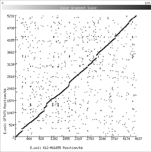
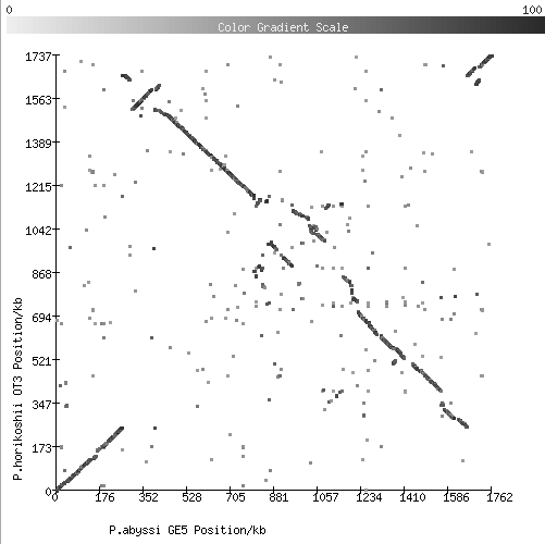
Genome Dot Plots
The following plots were generated using CMR Protein Scatter Plot tool.Synteny - gene order conservation along a chromosome.
1. Comparison of two strains of E.coli:
2. Comparison of two species of Pyrococcus (archaea):
3. Comparison of two strains of Prochlorococcus marinus (marine cyanobacteria):
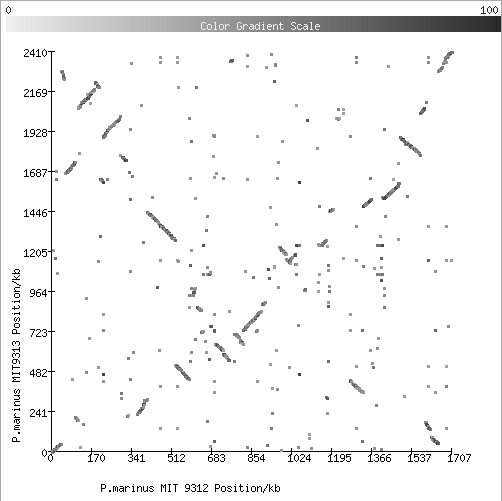
For discussion of observed patterns like that click here (see Fig.2 in particular).
ORFans, group-specific genes and Genomic Islands
ORFan - a gene with no detectable homologs in database. Visit the ORFanage here or here. According to the latter source, there are 68770 ORFans in 330 genomes.ORFans as the result of viral horizontal gene transfer: pros and cons.
BLAST atlases (see your reading material for the previous class: Figure 7)
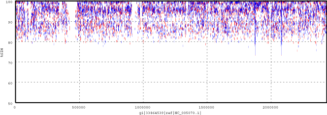
Identification of Genomic Islands: Synechococcus sp. WH8102 vs. Sargasso Sea MUMmerplot (alignment of Sargasso Sea reads against the genome of this marine cyanobacterium)
Clusters of Orthologous Groups (COGs)
[Alternative - TIGR Families]
BLASTology blunders
Example: bacterial genes in human genome: In the article on the "Initial sequencing and analysis of the human genome", 113 genes were claimed to be putative instances of horizontal gene transfer from Bacteria to vertebrates based on BLAST analyses."An interesting category is a set of 223 proteins that have significant similarity to proteins from bacteria, but no comparable similarity to proteins from yeast, worm, fly and mustard weed, or indeed from any other (nonvertebrate) eukaryote. These sequences should not represent bacterial contamination in the draft human sequence, because we filtered the sequence to eliminate sequences that were essentially identical to known bacterial plasmid, transposon or chromosomal DNA (such as the host strains for the large-insert clones). To investigate whether these were genuine human sequences, we designed PCR primers for 35 of these genes and confirmed that most could be readily detected directly in human genomic DNA (Table 24). Orthologues of many of these genes have also been detected in other vertebrates (Table 24). A more detailed computational analysis indicated that at least 113 of these genes are widespread among bacteria, but, among eukaryotes, appear to be present only in vertebrates. It is possible that the genes encoding these proteins were present in both early prokaryotes and eukaryotes, but were lost in each of the lineages of yeast, worm, fly, mustard weed and, possibly, from other nonvertebrate eukaryote lineages. A more parsimonious explanation is that these genes entered the vertebrate (or prevertebrate) lineage by horizontal transfer from bacteria."
Responses to the claim:
Microbial genes in the human genome: lateral transfer or gene loss?
Are there bugs in our genome?
Steps of the phylogenetic analysis:
| Compilation of sequence dataset |
| Alignment |
| Determination of substitution model |
| Tree building |
| Tree evaluation |
- Compilation of sequence dataset. It only makes sense to analyze homologous sequences. For example, use BLAST or COGs.
- Alignment. Sequence alignment is a line-up of two or more homologous sequences. Since in the course of evolution not only mutations, but
insertions and deletions occur (INDELs), the alignment algorithm(s) insert(s) gaps into some sequences:
For further analyses, choose only reliable parts of an alignment! - Choose a model of evolution. In order to reconstruct the evolutionary history of the sequences, we need to know how sequences evolved.
Examples:
- Jukes-Cantor's (JC69) model: equal frequency of nucleotides, each substitution is equally probable.
- Models that take into account transition/transversion bias (Kimura's 2-parameter model) and nucleotide frequencies (e.g., HKY85)
- Correction for Among Site Rate Variation (can be modelled with Gamma distribution) and proportion of invariable sites
Which model fits your data? There are programs that help to choose the best-fit model: MODELTEST ("...program for the selection the model of nucleotide substitution that best fits the data. The program chooses among 56 models...")
- Tree building or tree search. Three main methodologies: distance methods (calculate tree based on observed distances),
parsimony methods (find the tree that explains sequence data with minimum number of substitutions), and maximum likelihood methods (given a model for sequence evolution, find the tree that has the highest probability under this model).
Number of phylogenetic trees. - Tree evaluation. It is important to consider artifacts that might originate in phylogenetic reconstruction, and to assess the reliability of your results.
